This problem relates to Backpropagation algorithm used in training Neural Networks. The Backpropagation algorithm learns by calculating the gradient at each layer of the network starting from the last (near to output) going backwards. Sometimes these gradients can tend to be zero or become really huge numbers resulting in difficulty in training the network i.e. it becomes impossible to calculate the weights that will reduce the loss function and converge towards the global optima. The problem of gradients becoming zero is called Vanishing gradients whereas the when the gradients become really huge is called Exploding gradients. This problem can collectively be called unstable gradients.
This behavior which was observed in early 2000s that was one of the reasons that Neural Networks were mostly abandoned. If you want to know the details on what causes this, you can read the 2010 paper by Xavier Glorot and Yoshua Bengio.
Root Cause
Glorot and Bengio found sigmoid activation function and the weight initialization technique using normal distribution (mean 0 and std deviation of 1) as the main culprits. This configuration of the network resulted in the variance of the outputs of each layer to be much greater than the variance of its inputs. Therefore, in the forward pass the variance keeps increasing after each layer until the activation function (sigmoid) saturates at the top layers.
The Sigmoid activation function saturates at 0 or 1 when the inputs become really large, that results in derivatives close to 0. Therefore when the backpropagation kicks in it has virtually no gradient to propagate back through the network.
Remedies
1. Use different Initialization strategies
In the same paper Glorot and Bengio, proposed a way to significantly reduce the unstable gradients problem. In order to flow the signal properly in both directions (forward pass and backward propagation), without letting the signal to die out, we need the variance of outputs of each layer to be equal to the variance of its inputs and we need gradients to have equal variance before and after flowing through a layer in the reverse direction. There is a tradeoff here as it is not possible to guarantee both unless the layer has an equal number of inputs (fan-in of the layer) and outputs(fan-out of the layer).
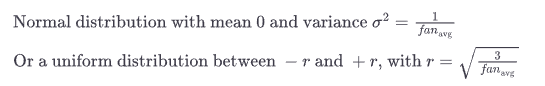
But the authors have proposed a good compromise that has proven to work very well in practice. The connection weights of each layer must be initialized randomly as described in equation below (when using sigmoid activation function) where fan_avg = (fan_in + fan_out)/2. This initialization strategy is called Xavier initialization or Glorot Initialization.
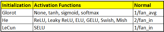
By default Keras uses Glorot initialization with a uniform distribution. You can change it by setting kernel_initialization parameter to “he_uniform” for ReLU activation function
import tensorflow as tf
dense = tf.keras.layers.Dense(50, activation="relu",<br>kernel_initializer="he_normal")
Alternatively, you can also obtain any of the initialization listed above and more using the VarianceScaling initializer as shown in the code below
he_avg_init = tf.keras.initializers.VarianceScaling(scale=2., mode="fan_avg",
                                                    distribution="uniform")
dense = tf.keras.layers.Dense(50, activation="sigmoid",
                              kernel_initializer=he_avg_init)
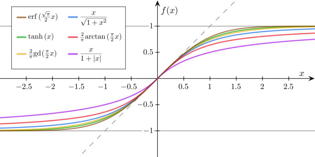
2. Use better Activation Functions
As Glorot an Bengio pointed out that one of the reason for unstable gradients was the commonly used sigmoid activation function, therefore researchers looked for other activation functions. Some of the most important ones that are better than sigmoid are mentioned below:-
Relu
It does not saturate for positive values and is also very fast to compute.
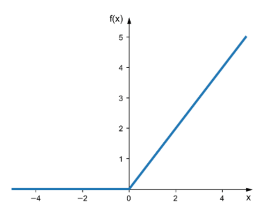
It suffers from a problem called dying ReLUs, because during training time some neurons effectively die which means they stop outputting anything other than zero. This problem gets worse if you use a large learning rate.
To solve this you may look at another variant of Relu – the leaky Relu as described below
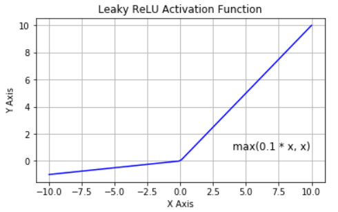
Leaky Relu
Instead of outputting zero for z<0 it outputs some negative value as defined by the hyperparameter Alpha. This parameter defines how much does the activation function leaks for z<0. In experiments setting alpha=0.2 (huge leak) performed much better than alpha=0.01 (small leak)
There is also a variant of leaky Relu called Randomized leaky Relu (RRelu) where alpha is picked randomly in a given range during training and is fixed to an average value during testing.
Another variant is parameterized Leaky Relu (PReLU), where alpha is learned during training, instead of being a hyperparameter. PReLU is reported to outperform strongly ReLU on large image datasets.
All variants of ReLU suffer from the problem that their derivatives change abruptly at z=0, that means they are not smooth. It can make gradient descent bounce around the optimum and slow down convergence.
Therefore now we will look at ELU and SELU which are smooth variants of Relu activation function.
ELU and SELU
ELU – In 2015 Clevert et al proposed exponential linear unit (ELU), that outperformed all ReLU variants where training time was reduced and the neural network performed better on the test set. ELU function looks a lot like the ReLU function but with the following major differences:-
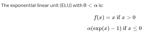
- The hyperparameter alpha defines the opposite of the value that the ELU function approaches when z is a very large negative number. It is usually set to 1 but you can tweak it like any other hyperparameter
- I has non zero gradient for z<0 which avoids the dead neuron problem
- The function is smooth everywhere including z=0, which helps speed up the gradient descent, since it does not bounce around to the left or right of z= 0
Main drawback:– Slower to compute than ReLU and its variants. It is due to the use of exponential function. However it has a faster convergence rate during training that may compensate for slow computation, but still at test time an ELU network will be a bit slower than ReLU network
SELU – Scaled version of ELU. It enables the network to self normalize, i.e. output of each layer tends to have mean of 0 and a standard deviation of 1 during training, that solves the vanishing/exploding gradient problem. But it requires following conditions to be met for self-normalization to happen
- Input features must be standardized to mean 0 and standard deviation of 1
- All Hidden layer weights must be initialized with LeCun normal initialization.
- Self normalization is only guaranteed with plain MLPs (multi layer perceptrons). It does not work well with RNNs, Skip Connections( Wide and Deep Nets)
- Regularization techniques like L1 or L2, max-norm, batch-norm or regular dropout cannot be used
Due to these significant constraints, SELU did not gain a lot of traction. Hence we will look at other activation function like GELU, Swish and Mish below which outperform SELU consistently

GELU, Swish, Mish
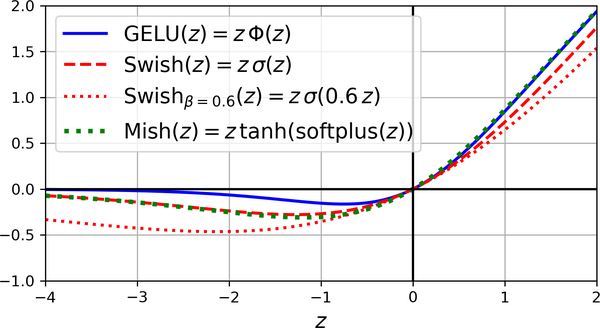
GELU – It was introduced in 2016 by Hendrycks and Gimpel. It is again a smooth variant of ReLU activation function. It resembles ReLU. It approaches 0 when its input is very negative, and it approaches z when z is very positive. However, whereas all the other activation functions discussed till now were both convex and monotonic, GELU is neither. It has a fairly complex shape and because it has a curvature at every point is the reason why it works so well as gradient descent may find it easier to fit complex patterns. In practice it outperforms all the activation functions discussed so far.
But it is a but more computationally intensive and may not justify the cost for the performance boost it provides.
Swish – Ramachandra et al discovered sigmoid linear unit (SiLU) which he named Swish where Swish = z * sigma(Beta * z) where Beta is the hyperparamter to scale the sigmoid function’s input. GELU is approximately equal to generalized Swish function using Beta = 1.702. It is also possible to make Beta trainable.
Mish – Another similar function is Mish which was inroduced by Diganta Misra in 2019. Just like GELU and Swish, it is a nonconvex, smooth and nonmonotonic variant of ReLU and outperformed all other activation functions even Swish and GELU (by a tiny margin). Mish overlaps almost perfectly with Swish when z is negative, and almost perfectly with GELU when z is positive.
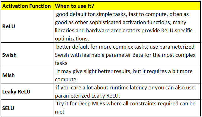
So which activation function to use?
3. Use Batch Normalization
Even after using He Initialization and Relu (or its variants) activation functions, which reduces the chances of vanishing and exploding gradient problem at the beginning of the training, the problem can still come back during training.
To avoid this Sergey Ioffe and Christian Szegedy proposed a technique called Batch Normalization in their 2015 paper. They proposed to add a normalization operation just before or after the activation function of each hidden layer. This operation will simply zero-center and normalize each input, then scales and shifts the results using two new parameter vectors per layer (one for scaling and another for shifting). This means that this operation lets the model learn the optimal scale and mean of each layer’s inputs. As this operation takes place over the current mini-batch, it is called the Batch normalization.
In order to zero center and normalize the inputs, the algorithm needs to estimate each input’s mean and standard deviation. The whole BN operation is summarized in the four steps below
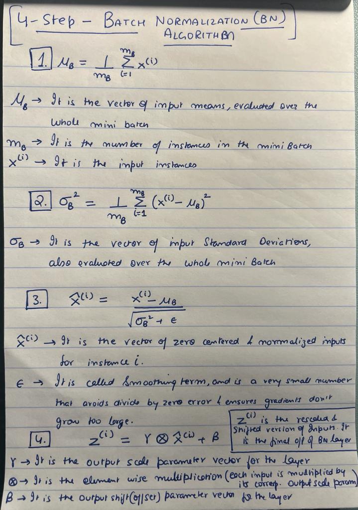
Batch Normalization at Test Time
BN standardizes, rescales and offsets its inputs in mini-batches, but at test time while making predictions the input does not come in batches, hence it becomes impossible to compute each input’s mean and standard deviation.
To resolve this issue at test time, BN estimates the final mean and standard deviation of inputs during training by using exponential moving average to calculate Mu (final input mean vector) and Sigma(final input standard deviation). Both Mu and Sigma are estimated during training but they are only used after training to replace the batch input means and standard deviations.
Batch Normalization at Run Time
Due to the fact that Batch Normalization increases the complexity of the model, the network suffers from a runtime penalty where it makes slower predictions. This is because extra computations are required at each layer. However Fusing the BN layer with previous layer’s weights can avoid this runtime penalty.
This fusing of weights updates the weights and biases of the previous layer so that it directly produces the output of appropriate scale and offset. TFLite’s converter automatically does this fusing operation.
Implementing Batch Normalization using Keras
It is very simple to implement Batch Normalization in Keras, you just need to add a BN layer before and after each hidden layer’s activation function, like in the example below
model = tf.keras.Sequential([
    tf.keras.layers.Flatten(input_shape=[28,28]),
    tf.keras.layers.BatchNormalization(),
    tf.keras.layers.Dense(300, activation="relu",kernel_initializer="he_normal"),
    tf.keras.layers.BatchNormalization(),
    tf.keras.layers.Dense(100, activation="relu",kernel_initializer="he_normal"),
    tf.keras.layers.BatchNormalization(),
    tf.keras.layers.Dense(10,activation="softmax")
])
You can also add BN layer as the first layer but a plain Normalization layer also works just as well in this location. Batch Normalization layer can make a huge difference in deeper networks.
Let’s analyze the model summary of the network we created above:-
Model: "sequential_1"
_________________________________________________________________
 Layer (type)                Output Shape              Param #
=================================================================
 flatten_1 (Flatten)         (None, 784)               0

 batch_normalization_3 (Batc  (None, 784)              3136
 hNormalization)

 dense_3 (Dense)             (None, 300)               235500

 batch_normalization_4 (Batc  (None, 300)              1200
 hNormalization)

 dense_4 (Dense)             (None, 100)               30100

 batch_normalization_5 (Batc  (None, 100)              400
 hNormalization)

 dense_5 (Dense)             (None, 10)                1010

=================================================================
Total params: 271,346
Trainable params: 268,978
Non-trainable params: 2,368
As you can see each BN layer adds four parameters per input i.e. Gamma (Output Scale), Beta (Output Offset or Shift) , Mu (Input means) and Sigma (Input std. deviations). That’s why you see 3136 (784 * 4) parameters in the second layer. Both Mu and Sigma are not affected by backpropagation and are simply moving averages, therefore Keras calls them non-trainable.
You can also check which are trainable and which are non-trainable parameters in the first BN layer using below command
[(var.name, var.trainable) for var in model.layers[1].variables]

Output:-
[('batch_normalization_3/gamma:0', True),
 ('batch_normalization_3/beta:0', True),
 ('batch_normalization_3/moving_mean:0', False),
 ('batch_normalization_3/moving_variance:0', False)]
The first two are True, hence trainable whereas last two are not. BN layer also has many hyperparameters that can be tweaked, two of the most important are the momentum and axis
momentum :- It is used when BN layer updates the exponential moving averages. A good momentum value is close 1, for example 0.9,0.99,0.999. The larger the datasets more 9’s you need
axis :- It determines which axis should be normalized. By default it is set to -1 which means the last axis is normalized. But you can set this value for example axis=[1,2] to treat each of the axis independently in a 2D batch.
Batch Normalization is one of the most used layers in Deep Neural networks especially in Convolutional Neural Networks (CNNs). It also acts like a regularizer and reduces the need for adding other regularization techniques such as dropout.
4. Use Gradient Clipping
This one is specifically for exploding gradients where gradients are clipped during backpropagation so that they never exceed some threshold. This technique is generally used in Recurrent Neural Networks where using batch normalization is tricky.
Implementing Gradient Clipping in Keras
It is just a matter of setting clipvalue or clipnorm arguments when creating the optimizer. Example below
optimizer = tf.keras.optimizers.SGD(clipvalue=1.0)
model.compile (...,optimizer=optimizer)
This optimizer will clip every component of the gradient vector to a value between -1.0 and 1.0. You can also tune this threshold as a hyperparameter. But you need to be careful as this clipping by value can change the direction of the gradient vector. For ex if your gradient vector is [0.9,90] which points mainly towards second axis, may point diagonally after clipping by value [0.9,1.0]. Therefore if you want to avoid this you can use clipnorm instead, that will not change the direction of the gradient vector. Because it will clip the whole gradient, if its L2 norm is greater than the threshold you picked.
You can use Tensorboard to observe if gradients are exploding during training by tracking the size of gradients. Then you can try clipping by value or norm, with different thresholds and see which option performs best on the validation set.
Conclusion
In this article we covered the problem of vanishing and exploding gradients while training Neural Networks. We understood the root cause and also looked at various ways to mitigate this problem. You can dive even deeper into this topic by going through the research papers linked in the text above. Do let me know in the comments below if you have any more questions on this topic